
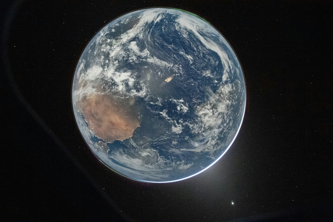
How a Signal Gets from Your Antenna to the Other Side of the World
Every amateur contact is a small act of applied physics. You press the key or speak into the microphone, and a few watts of electrical energy leave the antenna as an electromagnetic wave. What happens next, whether that wave dies a few miles from your house, bounces off the sky and lands in another continent, or gets swallowed by the atmosphere. This is the subject of “propagation”.
Propagation is the study of the path a radio signal takes between two points. It is part science, part weather-watching, and part experience. Two stations with identical equipment can have wildly different results on the same day, because the medium between them is constantly changing. The ionosphere breathes with the sun, the troposphere churns with the weather, and the geomagnetic field deflects streams of charged particles. Learning to read those changes is what turns operating from guesswork into strategy.
This article explains the main propagation mechanisms an amateur is likely to encounter, from the ground wave at 160 meters to moonbounce at 23 centimetres. It is written to be understood without a physics degree, but it does not shy away from the real mechanisms. Because these mechanisms are what make the hobby interesting.
1. The Medium: Earth’s Atmosphere and the Ionosphere
Radio waves travel through the atmosphere almost as easily as light travels through air. The lower atmosphere is electrically neutral: its molecules are not ionised, so it barely affects a passing wave. That is why VHF and UHF signals travel in essentially straight lines and disappear over the horizon.
The interesting part of the atmosphere is much higher up.
The layers of the atmosphere
The ionosphere is the region where the atmosphere is thin enough, and the solar radiation energetic enough, that a significant fraction of atoms and molecules have been stripped of one or more electrons. The result is a gas of free electrons and positive ions — a plasma. And a plasma, unlike neutral air, bends radio waves.
| Region | Approximate altitude | Relevance to radio |
|---|---|---|
| Troposphere | 0–12 km | Weather, temperature inversions, VHF/UHF ducting and scatter |
| Stratosphere | 12–50 km | Ozone layer; little direct effect on radio |
| Mesosphere | 50–85 km | Meteors burn up here; lower edge of the ionosphere |
| Thermosphere | 85–600 km | The ionosphere* lives here; satellites and the ISS orbit within it |
How the ionosphere is made
Sunlight contains extreme ultraviolet (EUV) and X-ray photons. When these photons strike atoms and molecules in the upper atmosphere, they knock electrons free. This process is called photoionisation. The rate at which it happens depends on:
– The intensity of sunlight: which varies with the solar cycle, the season, and the time of day.
- The density and composition of the atmosphere: at each altitude.
- The angle of the sun: a low sun delivers less energy per unit area.
At the same time, free electrons are constantly being lost through recombination, when an electron meets a positive ion and they neutralise each other. The balance between ionisation and recombination determines how many free electrons are present at any moment.
This balance explains the basic rhythm of the ionosphere. During the day, ionisation outruns recombination and electron density builds up. After sunset, the source of ionisation disappears and recombination takes over. But recombination is much faster where the gas is dense (at low altitude) and much slower where the gas is thin (at high altitude). That is why the lower layers vanish at night while the highest layer survives until dawn.
The ionospheric layers
The ionosphere is not a single uniform shell. It has a layered structure, named (from the bottom up) D, E, F1, and F2. The layers are not sharp boundaries; they are broad regions of enhanced electron density, and they change continuously with time, season, and solar activity.
| Layer | Altitude | Present | What it does |
|---|---|---|---|
| D | ~60–90 km | Daytime only | Absorbs HF signals, especially on the lower bands. Rapidly disappears after sunset. |
| E | ~90–120 km | Daytime; weak at night | Refracts signals for short-skip contacts. Also produces “sporadic E.” |
| F1 | ~150–220 km | Daytime, most pronounced in summer | A transition layer; merges into the F region at night. |
| F2 | ~250–500 km | Day and night | The main layer for long-distance HF communication. Highest electron density; survives the night. |
The F2 layer is the star of HF DX. It is high enough that a signal can travel a long way before returning to Earth, and it persists through the night, which is why 20 metres can still be open at midnight during a good part of the solar cycle. The D layer, by contrast, is the villain of the lower bands: it sits low, where the air is dense, and it converts radio energy into heat with ruthless efficiency.
A useful mental model: the D layer is a filter, the F layer is a lens. The lower bands must get through the D layer to reach the F layer; the higher bands punch through the D layer easily but need a strong F layer to bend them back.
2. What Can Happen to a Radio Wave
Once a wave leaves the antenna, one of four things happens to it:
1: it is absorbed
2: it is refracted
3: it is scattered
4: or it keeps going into space.
The relative importance of these depends on frequency, angle, and the state of the ionosphere.
Absorption
Absorption happens when a radio wave’s oscillating electric field accelerates free electrons, which then collide with neutral molecules and lose energy as heat. The effect is strongest where there are many electrons and many neutral molecules, that is, low in the ionosphere, in the D layer.
Two rules follow, and they explain a great deal of everyday operating:
1. “Absorption increases as frequency decreases”. Roughly, it scales as 1/*f*². This is why 80 meters is noisy and difficult in broad daylight while 20 meters sails through.
2. “Absorption depends on the sun”. It peaks near local noon and is negligible at night. It also increases during solar flares, which is why a flare can wipe out HF communication on the sunlit side of the Earth.
Refraction — the “reflection”
Amateurs habitually say a signal “bounces off the ionosphere.”, You will often hear that just called “Bounce”. It does not, strictly speaking, bounce. A mirror reflects; the ionosphere refracts. The difference matters, because it explains why propagation depends on frequency and angle in the way it does.
Plasma has a refractive index that is less than one and depends on the electron density and the wave frequency:
n² = 1 − (f_p / f)²
where f_p is the plasma frequency, a measure of how much electron density is present. As a wave travels upward into denser plasma, the refractive index falls. If the wave is travelling obliquely, the change in refractive index bends it gradually. If the gradient is strong enough and the angle shallow enough, the wave is bent all the way back down toward Earth. This is total internal reflection, the same effect that keeps light trapped inside an optical fibre.
Two consequences are worth remembering:
1: Higher frequencies need more electrons to be bent back. If the frequency is too high, the wave passes straight through the ionosphere and out into space.
2: Oblique paths can use higher frequencies than vertical paths. The shallower the angle at which the wave enters the layer, the more bending it gets per unit of electron density.
Critical frequency, MUF, and LUF
Three numbers describe the usable window on any given path.
1: Critical frequency (foF2). The highest frequency that the F2 layer will reflect straight back down when a signal is sent vertically. It is a direct measure of peak electron density and is typically 3–8 MHz at night and 5–12 MHz or more during the day, depending on the solar cycle.
2: Maximum Usable Frequency (MUF). The highest frequency that can be used for a path at a given angle. For a simple flat-layer approximation:
MUF ≈ foF2 × sec θ
where θ is the angle of incidence measured from vertical. A shallower angle (larger θ) means a larger secant and a higher MUF. For a 3,000 km path with the F2 layer at about 300 km, the angle is steep enough that the MUF can be roughly five times foF2. Forecasters often quote “MUF(3000)F2”, the MUF for a 3,000 km path, as a standard index.
3: Lowest Usable Frequency (LUF). The lowest frequency that will get through. It is set not by refraction but by absorption in the D layer. Go too low and the signal is simply absorbed before it reaches the F layer.
Between the LUF and the MUF lies the usable window. In practice, operators aim a little below the MUF at the Frequency of Optimum Traffic (FOT), often taken as about 85% of the MUF, because near the MUF the path is marginal and easily disturbed.
If the MUF is below the LUF, the band is closed. That is what “the band is dead” usually means: not that the ionosphere has vanished, but that no frequency satisfies both conditions.
Skip distance and the skip zone
A signal launched at a low angle travels a certain distance before it returns to Earth. The minimum distance at which a skywave returns is the “skip distance”. Between the end of reliable ground-wave coverage and the skip distance lies the “skip zone”. A ring of silence where neither the ground wave nor the skywave reaches.
The skip distance depends on frequency and layer height. Higher frequencies and higher layers produce longer skips. Until the frequency is so high that the wave punches straight through the layer and no skywave returns at all. This is why, on 40 meters during the day, you may hear stations 800 km away but nothing at 200 km. The near stations are inside your skip zone.
Multi-hop propagation
A skywave that returns to Earth can reflect off the ground and set off again. Each “hop” can span roughly 2,000 – 4,000 km on the F layer, so two or three hops can circle much of the planet. Each ground reflection costs some signal, and each pass through the D layer costs more, so multi-hop signals are weaker and more fluttery than single-hop ones.
Occasionally, a signal can make a chordal hop: it refracts in the F layer, travels some distance within the ionosphere, and refracts again without touching the ground. This produces unusually long single-hop distances and is one reason why some paths are unexpectedly strong.
3. The Bands and What They Do
Amateur bands are often described by wavelength rather than frequency, which is convenient because wavelength and propagation behaviour track each other closely. The rule of thumb is simple:
Lower frequency = more reliable, more absorbed, more noise.
Higher frequency = more fragile, less absorbed, more dependent on the sun.
For more details on what bandwidths and functions are please look at the Bandplan.
A rough operating heuristic:
– 160/80 m: Night, winter, and the grey line.
– 40 m: The reliable all-rounder; day for regional, night for DX.
– 20 m: The default DX band whenever the sun is reasonably active.
– 15/12/10 m: Daytime DX when the solar flux is high; sporadic E in early summer.
– 6 m and up: Seasonal, weather-dependent, and often surprising.
The higher bands are not “better.” They are simply more sensitive to the ionosphere. When conditions are right, 10 meters can deliver a contact 15,000 km away with a few watts. When conditions are wrong, it is silent for weeks. The lower bands are the opposite: always something to hear, rarely spectacular.
4. Skywave in Detail
Skywave: A refraction by the ionosphere. This is the mechanism behind most long-distance amateur contacts. Within skywave there are several distinct sub-modes worth knowing.
F2 long-distance DX
The classic DX path: a signal leaves the antenna at a low angle, passes through the D and E layers, refracts in the F2 layer, and returns to Earth hundreds or thousands of kilometres away. At solar maximum, 10 meters can support this with modest power; at solar minimum, 20 meters may struggle.
The key variable is takeoff angle. A low angle (a few degrees above the horizon) produces a long single hop and is essential for extreme DX. That is why DX antennas are designed for low-angle radiation: tall verticals, Yagis on high towers, and Beverage antennas for the low bands.
NVIS — Near Vertical Incidence Skywave
NVIS is the opposite of DX. The signal is launched almost straight up, refracts in the F layer, and comes back down within a few hundred kilometres. It fills in the skip zone and is the standard technique for regional communication in mountainous or remote areas, and for emergency communications.
NVIS works best on frequencies ‘below the critical frequency’. Typically 40 meters during the day and 80 meters at night. With an antenna that radiates at a high angle. A horizontal dipole mounted only a fraction of a wavelength above ground is ideal, because the ground reflection reinforces the high-angle lobe. A vertical antenna is a poor NVIS choice: it radiates toward the horizon.
The practical range is roughly 0–500 km, sometimes a little more, and the signal is often strong and stable — much less prone to fading than a long DX path.
Grey line
The “grey line” is the terminator, the moving boundary between day and night. Along it, the D layer is fading away while the F layer is still ionised. For a short window, low-band signals can travel a long way with unusually low absorption.
Grey-line DX is one of the most satisfying aspects of the hobby. On 80 and 160 meters, contacts of 5,000–10,000 km become possible around sunrise and sunset, especially when the path runs along the terminator. The effect lasts tens of minutes, not hours, so timing matters. Many operators use grey-line maps or calculators to plan.
Long path
The shortest great-circle route between two stations is the “short path”. The opposite direction, halfway around the world, is the “long path”. Long-path signals can be strong when the geometry and the terminator favour the longer route. Often around sunrise or sunset, when one route lies along the grey line and the other does not.
Long path is a favourite of experienced DXers because it can produce contacts that are impossible on the short path, and because signals arrive with a distinctive echo or flutter as the two paths interfere.
Trans-equatorial propagation (TEP)
TEP occurs on paths that cross the geomagnetic equator, particularly on 6 and 2 meters. It is associated with equatorial ionospheric anomalies and is strongest in the evening during high solar activity. Distances of 4,000–8,000 km are possible on 6 meters, which is remarkable for a band that normally behaves like VHF.
Spread F and ionospheric irregularities
The ionosphere is not a smooth, flat layer. It contains irregularities. patches, bubbles, and travelling disturbances, that scatter and distort signals. Equatorial spread F is a common cause of flutter and deep fading on low-latitude paths in the evening. Travelling ionospheric disturbances (TIDs) produce slow, rhythmic fading. These effects are a reminder that the ionosphere is a dynamic, three-dimensional medium, not a set of concentric shells.
5. Beyond Skywave: Other Propagation Modes
Skywave is the main event on HF, but it is not the only way a signal can travel. Several other mechanisms matter, especially above 30 MHz.
Ground wave
A ground wave, hugs the surface of the Earth, following its curvature by diffraction. It is strongest at low frequencies and over good conductors. Seawater is excellent, dry sandy soil is poor. On 160 and 80 meters, the ground wave provides reliable local coverage out to tens of kilometres, and on the broadcast band it reaches much further.
At VHF and UHF, the ground wave is essentially line-of-sight, with a little diffraction over obstacles. This is why repeater coverage is described in terms of terrain and antenna height rather than ionospheric conditions.
Sporadic E (Es)
Sporadic E is the appearance of intense, patchy ionisation in the E layer, typically at 90–120 km. The patches are small (tens to hundreds of kilometres across), drift with the wind, and can support refraction at frequencies far above the normal E-layer limit — often up to 50 MHz, occasionally 144 MHz.
Sporadic E is strongly seasonal in the northern hemisphere: it peaks in late spring and early summer (May–July), with a smaller peak around midwinter. It is also more common in the late morning and early evening. A single Es hop can span roughly 2,000 km on 6 meters; double-hop contacts of 4,000 km or more are recorded every season.
For 10 and 6 meter operators, Es is the main source of excitement outside solar maximum. It is also a useful propagation indicator: when 10 meters opens to a single region for a few minutes and then vanishes, that is classic Es.
Tropospheric ducting and scatter
The troposphere. “The weather layer”, can also refract VHF and UHF signals. When a temperature inversion forms (warm air above cool air), the refractive index gradient can trap signals in a duct between the inversion and the ground or between two inversions. This tropospheric ducting can extend 2-metre and 70-centimetre range to 500–1,000 km or more, especially over water. You will often hear this referred to as “Tropo”.
Ducting is weather-dependent, not sun-dependent, and is most common in settled high-pressure systems, often in summer and autumn. Tropospheric scatter is a related effect: irregularities in the troposphere scatter a small fraction of the signal forward, allowing contacts at 300–800 km with high power and large antennas.
Meteor scatter
When a meteor enters the atmosphere, it leaves a trail of ionised gas that can reflect radio waves for a fraction of a second to a few seconds. Amateurs use these trails for meteor scatter contacts on 6 and 2 meters, typically over distances of 500–2,300 km.
The technique requires patience and the right tools: high power, a good antenna, and a digital mode such as MSK144 that can decode very short pings. Major annual showers like the Perseids in August, the Geminids in December, the Quadrantids in January, provide the best conditions, but sporadic meteors produce usable trails every day.
Auroral propagation
Aurora is caused by charged particles from the solar wind funnelling along geomagnetic field lines and colliding with the upper atmosphere. The resulting ionisation can refract VHF signals, but it does so with characteristic distortion: signals become “raspy, hollow, and fluttery”, because the auroral ionisation is irregular and moving.
Auroral contacts are made on 6 and 2 meters, usually when the KP index is 5 or higher. The geometry is unusual: stations point their antennas toward the aurora (roughly north in the northern hemisphere), and contacts are possible between stations at similar distances from the auroral oval. On HF, aurora causes absorption and flutter, particularly on high-latitude paths.
Earth–Moon–Earth (EME)
Moonbounce uses the Moon as a passive reflector. The round-trip path is about 768,000 km, and the round-trip path loss at 2 meters is roughly 400 dB. A staggering figure that explains why EME stations use high power, very large antennas, and extremely low-noise receivers.
Despite the difficulty, EME is a thriving part of the hobby on 2 meters, 70 centimetres, and 23 centimetres and above. Modern digital modes such as JT65 and Q65 can decode signals far below the noise floor, which has made moonbounce accessible to more stations than ever. The Moon’s libration and the Doppler shift from its motion add interesting complications.
Satellites and aircraft scatter
Amateur satellites. including the ISS, provide line-of-sight contacts on VHF and UHF, often over 2,000 km. Doppler shift is significant: roughly ±3 kHz on 2 meters and ±10 kHz on 70 centimetres, so operators tune continuously during a pass.
Aircraft scatter uses reflections from aircraft to extend VHF/UHF range by a few hundred kilometres, and rain scatter does something similar at microwave frequencies. Both are specialist techniques, but they illustrate a general point: almost any conducting or refracting object can redirect a radio wave if the geometry is right.
6. The Sun: The Engine Behind It All
If there is one thing to understand about HF propagation, it is this: The sun drives the ionosphere. Everything else: season, time of day, geomagnetic activity, is a modulation of that primary driver.
Sunspots and the solar cycle
Sunspots are regions of intense magnetic activity on the solar surface. They are cooler than their surroundings and appear dark, but they are associated with the strong EUV and X-ray emission that creates the ionosphere. More sunspots generally mean a more ionised ionosphere and better high-frequency propagation.
The sunspot number rises and falls over a period of roughly 11 years. Each cycle also reverses the sun’s magnetic polarity, so the full magnetic cycle is about 22 years. The solar flux index (SFI), measured at 10.7 cm wavelength, is a convenient proxy: values around 70 indicate solar minimum, 150 is a healthy active sun, and 200+ is exceptional.
Information on Sunspots and Solar weather can be tracked online at Spaceweather.
Solar Cycle 25 began in December 2019, peaked around 2024–2025, and is now in its declining phase. That means conditions will gradually move from the generous openings of solar maximum toward the quieter, more 20-metre-centric patterns of solar minimum. The practical lesson is to enjoy the high bands while they last and to build low-band capability for the years ahead.
Solar Flares, CMEs, and geomagnetic storms
The sun’s activity manifests in several ways that affect radio:
1: Solar flares: Are sudden releases of X-ray and EUV energy. They increase D-layer ionisation on the sunlit side of the Earth, causing sudden ionospheric disturbances (SIDs), short-wave fadeouts, that can last from minutes to a couple of hours. A strong flare can black out HF communication across an entire hemisphere. (The same effect improves VLF and LF propagation, which is why some amateurs monitor VLF stations to detect flares.)
2: Coronal mass ejections (CMEs): Hurl clouds of magnetised plasma into space. When one reaches Earth, it can trigger a geomagnetic storm, measured by the Kp index (0–9) and the A index. Storms degrade HF propagation at high latitudes, cause aurora, and produce deep fading. A severe storm can close the high-latitude HF paths entirely for a day or more.
3: Solar radiation storms: bursts of energetic protons that cause polar cap absorption (PCA), which blacks out HF paths through the polar regions for hours to days. These are a serious concern for transpolar routes.
Geomagnetic storms are not uniformly bad. They often improve low-latitude paths for a while (the “positive phase” of a storm) before depleting the F layer (the “negative phase”). They also open auroral paths on 6 and 2 metres. The net effect depends on latitude, time, and the storm’s structure.
Seasonal and daily patterns
The ionosphere follows the sun’s apparent motion:
– Day/night: The D layer appears at sunrise and vanishes at sunset; the F layer thins at night but persists. This is why the low bands come alive after dark and the high bands peak around local noon.
– Season: The equinoxes (March and September) generally favour DX, because the terminator is aligned with the meridian and both ends of a path can be in daylight or darkness together. Summer brings sporadic E and higher atmospheric noise; winter favours the low bands and often brings quieter geomagnetic conditions.
– The winter anomaly: Daytime F2 ionisation can actually be higher in winter than in summer, because the changed atmospheric composition favours electron survival. This is one of several reasons why winter is a good DX season on the higher bands too.
Space Weather Indices at a glance
Space weather indices at a glance
| Index | What it measures | Useful range |
|---|---|---|
| SFI (solar flux) | 10.7 cm radio emission; proxy for solar activity | 70 (low) to 200+ (high) |
| SSN | Sunspot number | 0 to 200+ |
| Kp | Planetary geomagnetic disturbance, 3-hourly | 0–3 quiet, 4 unsettled, 5+ storm |
| A index | Daily geomagnetic activity | 0–10 quiet, 20+ disturbed |
| Bz | North–south component of the interplanetary magnetic field | Sustained negative Bz favours storms |
| Solar wind speed | Speed of the solar wind at Earth | 300 km/s quiet, 600+ km/s disturbed |
A useful rule of thumb: high SFI is good for the high bands; low Kp is good for stable paths. A high SFI with a high Kp is a mixed blessing. The ionosphere is charged up but disturbed.
7. Reading the Weather: Forecasts and Tools
Propagation forecasting is not fortune-telling. It is a combination of physics-based models and real-time observations. Several free tools make it accessible.
VOACAP: the classic HF propagation prediction program, based on ionospheric models and path geometry. It produces charts of reliability versus frequency and time of day for a given path. It is the standard tool for planning DXpeditions and contests.
ITURHFPROP: the ITU’s reference implementation of the same kind of modelling.
Proppy: a web-based front end that makes VOACAP-style predictions easy to run for a specific path and date.
These models are only as good as their inputs. They assume a smooth, average ionosphere, so they are best used for planning rather than for moment-to-moment decisions.
Real-time observations
– WSPRnet: the Weak Signal Propagation Reporter network. Stations transmit very low-power beacons (often just a few hundred milliwatts) on a fixed schedule, and receiving stations report them. The resulting maps show, in near real time, exactly which paths are open on which bands. It is the single best tool for seeing propagation as it happens.
– Reverse Beacon Network (RBN): a network of automated skimmers that report callsigns heard on CW and digital modes, with signal strength and frequency. Excellent for contest and band-opening analysis.
– PSK Reporter: similar to RBN but for digital modes such as FT8, FT4, and PSK31.
– DXHeat / DX Maps: aggregators that display DX spots and live propagation maps.
– NCDXF/IARU beacon network: a set of 18 beacons transmitting in sequence on 14.100, 18.110, 21.150, 24.930, and 28.200 MHz, cycling through power levels from 100 W down to 100 mW. Listening to the beacons gives an instant, low-tech read on which bands are open and how well.
– NOAA Space Weather Prediction Center: the authoritative source for solar flux, Kp, solar wind, flare alerts, and aurora forecasts. Also provides D-RAP (D-Region Absorption Prediction) maps.
8. Practical Operating
Propagation knowledge is only useful if it changes what you do. Here are the habits that matter most.
Follow the sun
The single most reliable rule: work the band that is in daylight at both ends of the path, or the band that is in darkness at both ends. A path where one end is in bright sun and the other is in deep night is usually difficult on the higher bands, because the ionosphere is asymmetric.
Around sunrise and sunset, the terminator sweeps across the path, and the low bands can open briefly and strongly. This is the grey-line effect, and it is worth planning your operating around.
Match the antenna to the mode
– DX on HF: low takeoff angle. Verticals, Yagis on tall towers, and Beverage antennas for receive.
– NVIS: high takeoff angle. A low horizontal dipole or inverted-V. There is an example here.
– VHF/UHF weak signal: horizontal polarisation, high gain, low noise figure.
– FM repeaters and satellites: vertical polarisation, circular polarisation for satellites.
An antenna that is excellent for DX may be poor for NVIS, and vice versa. There is no single “best” antenna; there is only the best antenna for the path you want.
Manage noise
On the low bands, the limiting factor is often not signal strength but noise. Atmospheric noise (QRN) is high in summer and low in winter; man-made noise (QRM) is everywhere. A quiet receive antenna: a small loop, a Beverage, or a phased array can transform 160 and 80 metres. Noise cancelling and diversity reception help too.
Use the digital modes
This site has a comprehensive glossary of digital modes here.
FT8, FT4, WSPR, and their relatives have changed propagation study. They decode signals far below the noise floor, which means they can reveal openings that would be invisible to CW or SSB. A 10-watt FT8 contact on 6 metres during an Es opening is a perfectly ordinary event; the same contact on SSB might be impossible.
Digital modes are also the best propagation sensors: a station that is transmitting WSPR every two minutes is a continuous, automated probe of the ionosphere.
Watch the MUF, not just the band
If the MUF is 21 MHz, 15 metres may be marginal while 20 metres is solid. If the MUF is 28 MHz, 10 metres may be wide open. Learning to think in terms of “what is the MUF right now” rather than “is 10 metres open” makes you a better operator.
9. Experiments for the Curious
Propagation is an experimental science, and amateur radio is one of the few places where you can do real experiments with real equipment.

Leave a Reply
You must be logged in to post a comment.